Airborne Gravity with AIRGrav

Sander Geophysics Limited (SGL) offers airborne gravity surveys using our Airborne Inertially Referenced Gravimeter - AIRGrav.  SGL´s AIRGrav is the only purpose-built airborne gravimeter, and was designed specifically for the unique characteristics of the airborne environment.  This design approach has resulted in a superior gravity instrument which can be flown in an efficient survey aircraft during normal daytime conditions.  In addition, AIRGrav can easily be flown in combination with magnetic and/or radiometric instruments to increase the survey benefits.  AIRGrav was designed primarily for petroleum exploration, where it is an economical alternative to ground and shipborne surveys.  AIRGrav also has exciting application in regional geophysics, mineral exploration and geodesy.

The AIRGrav system includes an all new gravimeter on a three-axis inertially stabilized platform, combined with high resolution Differential GPS (DGPS) to correct for aircraft movements due to turbulence, aircraft vibrations and drape flying.  The gyro stabilized inertial platform makes the gravimeter much less affected by horizontal accelerations than other systems, which use modified sea gravimeters.  This allows AIRGrav to achieve consistently higher resolution.  The AIRGrav system is currently available to fly fixed-wing or helicopter surveys.

Terrain corrections are performed using either an existing digital terrain model or terrain data acquired in the course of the gravimetric survey.  Digital terrain models can be supplemented with remote sensing data if required, depending on the nature of the terrain and the resolution of the survey.  Terrain corrections for airborne gravity surveys are in some ways easier than ground surveys because airborne gravity does not require near station corrections, and is not susceptible to errors due to anomalous densities near a gravity station.

Production surveys have been flown under a variety of conditions including offshore, at a constant altitude over rolling terrain, and with a loose drape over high mountains (>3,000 m).  Because the system is relatively tolerant of turbulence, it works well on drape surveys and in moderate to severe turbulence.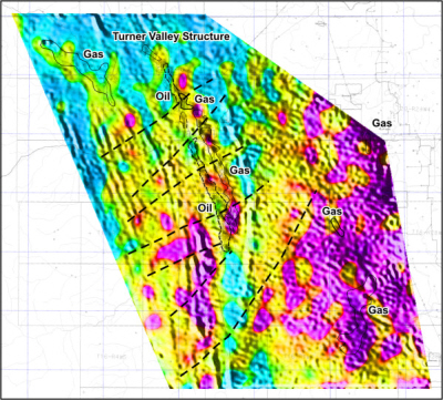

Sander Geophysics recently completed a combined gravity and magnetic survey in the Turner Valley area, south of Calgary, Canada.  The map above shows the first vertical derivative of the terrain corrected Bouguer gravity with the shadow of the first vertical derivative of the total magnetic intensity.  The data set consists of over 12,000 lkm of data flown on 250 m spaced east-west lines, and 1,000 m north-south lines. The extent of the data set is 60 km from north to south.  Noise was calculated to be 0.3 mGal.  Gravity anomalies of less than 2 mGal can be seen clearly on the data set and correlate well with known oil and gas fields.

Results from numerous AIRGrav surveys have been rigorously analyzed to determine system performance and optimum processing parameters.  The graph below shows rms gravity noise plotted against filter length (20 s = 1 km).  The graph shows that the noise level drops off quickly as the filter length increases, which indicates that noise is concentrated in the higher frequencies.  The graph also clearly illustrates the relationship between accuracy and resolution, and how one can be traded off against the other depending on the client´s objectives.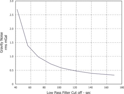

The following graph demonstrates the effect of averaging a number of lines (a process which is similar to stacking seismic data), which can be achieved by flying closely spaced lines and applying a filter with a wavelength longer than the line spacing.  The graph shows rms gravity noise plotted against the number of lines averaged, for various filter lengths.   Using this procedure, the final grid data will have a noise level significantly lower than the individual profile data.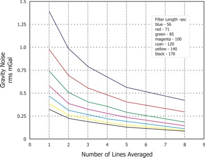

Shown below are typical AIRGrav survey parameters.  As described above, the accuracy and resolution of the gravity data depends on the aircraft speed and the line spacing.

AIRGrav services include survey planning, data acquisition, preliminary processing in the field, final data processing to terrain corrected Bouguer gravity and a comprehensive technical report.  SGL also offers integrated interpretation of AIRGrav, aeromagnetic and other data sets.